7.3. Rational Rate Conversion#
Consider interpolating \(x[n]\) by a factor \(U\) and then downsampling by a factor \(D\):
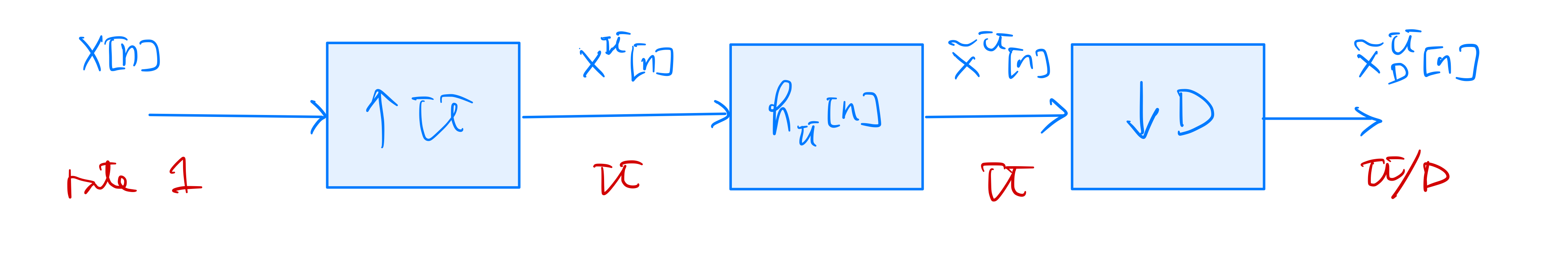
The rate of the output signal \(\tilde{x}^U_D[n]\) if \(\frac{U}{D}\) times that of the input \(x[n]\).
From (7.5), we get
\[\begin{align*} \tilde{x}^U_D[n] &= \tilde{x}^U[Dn] \\ &= \sum_{k=-\infty}^{\infty} x[k] \, \frac{\sin \left(\frac{\pi}{U/D} (n-k\frac{U}{D}) \right)}{\frac{\pi}{U/D} (n-k\frac{U}{D})}. \end{align*}\]If \(x[n]\) is obtained from oversampling a continuous-time signal \(x(t)\) at sampling rate \(f_s\), then based on the sampling theorem (3.9) sampling \(x(t)\) at rate \(f_s \frac{U}{D}\) gives
\[\begin{align*} x \left(\frac{n}{U f_s/D} \right) &= \sum_{k=-\infty}^{\infty} x[k] \, \frac{\sin \pi f_s \left(\frac{n}{U f_s/D} -\frac{k}{f_s} \right)}{\pi f_s \left(\frac{n}{U f_s/D} -\frac{k}{f_s} \right)} \\ &= \tilde{x}^U_D[n]. \end{align*}\]That is, \(\tilde{x}^U_D[n]\) is the sampled version of \(x(t)\) obtained at sampling frequency \(f_s \frac{U}{D}\).
Caution
Even though \(x[n]\) is obtained from oversampling \(x(t)\), \(\tilde{x}^U_D[n]\) may still suffer from aliasing due to the rate conversion process from \(x[n]\). See the discussion below for details.
Working backward from \(\tilde{x}^U_D[n]\) in the figure of the rate conversion system above, we can recover \(\tilde{x}^U[n]\) (and hence \(x[n]\)) if the downsampling process doesn’t suffer from aliasing, i.e., its DTFT \(\tilde{X}^U(e^{j\hat\omega}) = 0\) for\(\frac{\pi}{D} \leq |\hat\omega| \leq \pi\):
If \(U \geq D\), this oversampling requirement is automatically satisfied since \(H_U(e^{j\hat\omega}) = 0\) for \(\frac{\pi}{D} \leq |\hat\omega| \leq \pi\) in this case.
If \(U < D\), the oversampling requirement is satisfied only if \(\tilde{X}^U(e^{j\hat\omega}) = 0\) for \(\frac{\pi}{D} \leq |\hat\omega| \leq \pi\), which in turn implies the requirement of \(X(e^{j\hat\omega}) = 0\) for \(\frac{\pi U}{D} \leq |\hat\omega| \leq \pi\) because of (7.4).
For case 2, we may replace the ideal lowpass filter between the upsampler and downsampler with a combined interpolation and antialiasing ideal lowpass filter with frequency response \(\displaystyle H_{\max(U.D)}(e^{j\hat\omega}) = \begin{cases} U & \text{for } |\hat\omega| < \frac{\pi}{\max(U,D)} \\ 0 & \text{for } \frac{\pi}{\max(U,D)} \leq |\hat\omega| \leq \pi \end{cases}\)
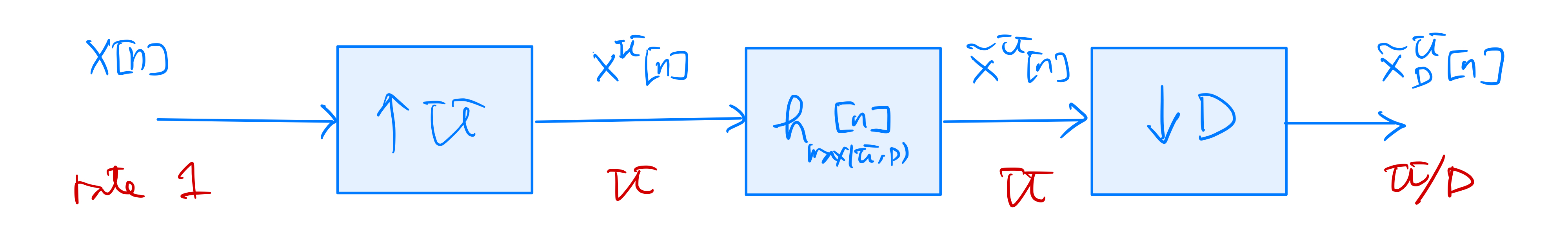
In practice, we have to approximate the ideal filter with a lowpass FIR or IIR filter with cutoff at \(\frac{\pi}{\max(U,D)}\). Note that this filter operates at the interpolated rate. The filter design techniques discussed in Section 6 can be employed to design this pratical interpolation-antialiasing filter.