7.5. Polyphase Decomposition & Related Identities

• We want to develop an efficient way to implement multi-rate filters. To that end, we start by introducing a number of simple algebraic results that help such a development.

7.5.1. Polyphase Decomposition Identity

• Let \(h[n] \stackrel{z}{\longleftrightarrow} H(z)\) be the impulse response and transfer function of an LTI filter. Fix a positive integer \(M\). Define

  (7.7)\[\begin{equation} e_k [n] = h[nM+k] \end{equation}\]

  for \(k=0,1,\ldots,M-1\). We may interpret that \(e_k[n]\) is obtained from downsampling \(h[n+k]\), which is referred to as a phase of \(h[n]\), by factor \(M\).

• Let \(e_k[n] \stackrel{z}{\longleftrightarrow} E_k(z)\). Then

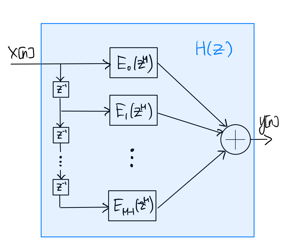
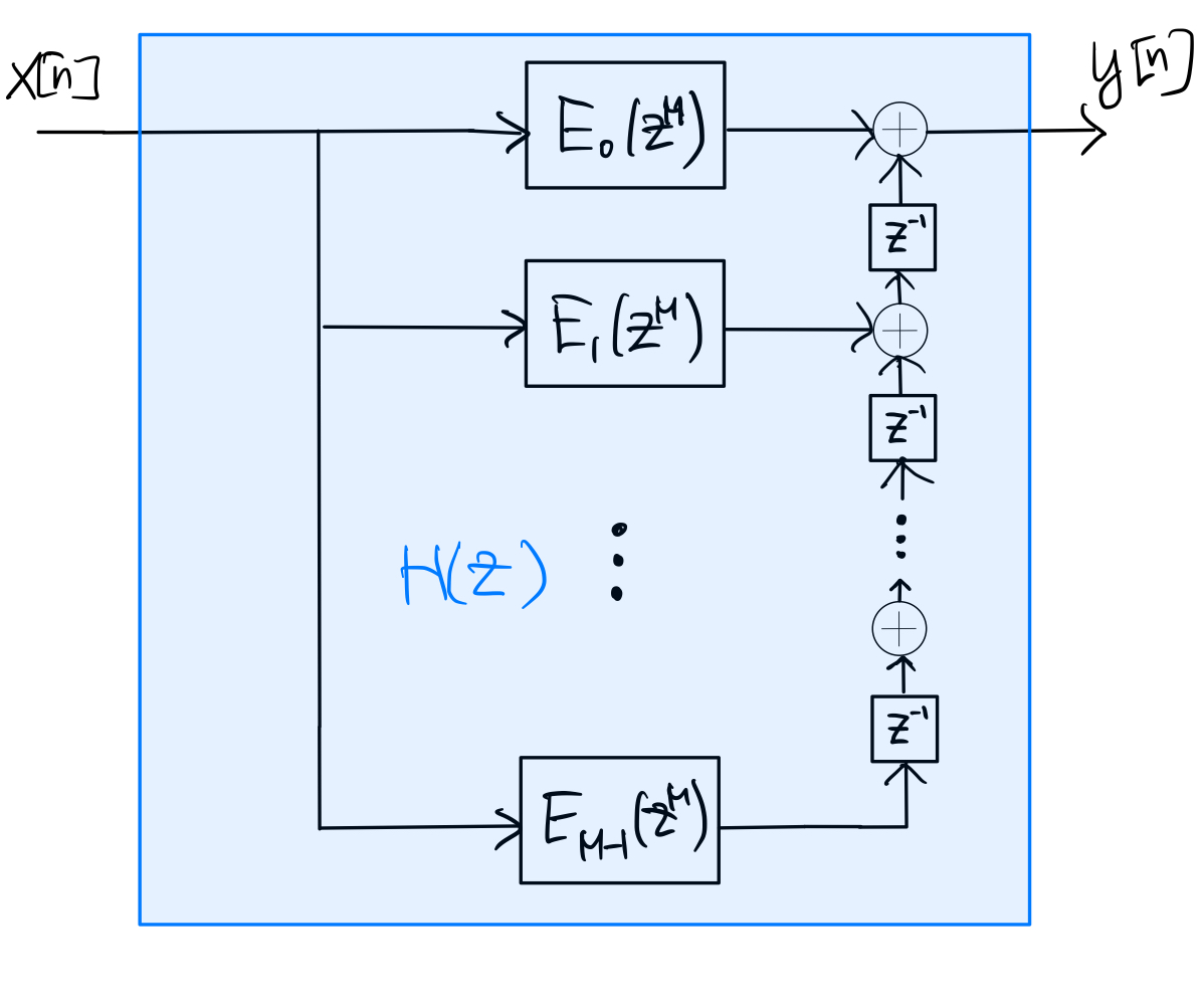
  (7.8)\[\begin{split}\begin{align} H(z) &= \sum_{n=-\infty}^{\infty} h[n] z^{-n} \\ &= \sum_{k=0}^{M-1} \sum_{m=-\infty}^{\infty} h[mM+k] z^{-(mM+k)} \\ &= \sum_{k=0}^{M-1} \left( \sum_{m=-\infty}^{\infty} e_k[m] z^{-mM} \right) z^{-k} \\ &= \sum_{k=0}^{M-1} z^{-k} E_k(z^M) \end{align}\end{split}\]

  which is called the polyphase decomposition of the filter \(H(z)\). It implies the following structures for implementing \(H(z)\):

  • Direct polyphase form:

    

  • Transposed polyphase form:

    

7.5.2. Downsampling Identity

• The following two systems are equivalent:

  

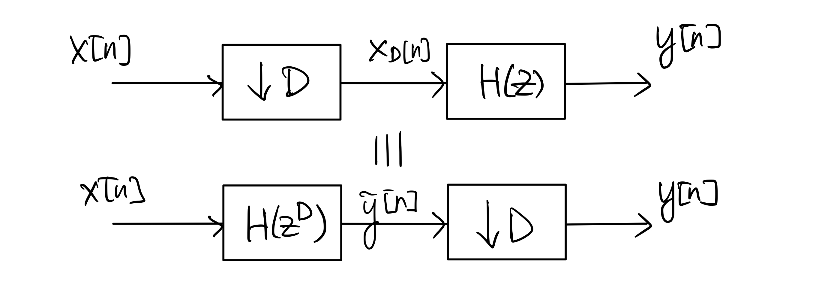
• We call the equivalence above the downsampling identity. It can be shown by first recalling from (7.1) that

  \[\begin{equation*} X_D(z) = \frac{1}{D} \sum_{k=0}^{D-1} X\left( e^{-j\frac{2\pi k}{D}} z^{\frac{1}{D}} \right). \end{equation*}\]

  Moreover, \(\tilde{Y}(z) = H(z^D) X(z)\) from the second system in the figure above. From the first system, we have

  \[\begin{align*} Y(z) &= H(z) X_D(z) \\ &= \frac{1}{D} \sum_{k=0}^{D-1} H(z) X\left( e^{-j\frac{2\pi k}{D}} z^{\frac{1}{D}} \right) \\ &= \frac{1}{D} \sum_{k=0}^{D-1} H\left( \left(e^{-j\frac{2\pi k}{D}} z^{\frac{1}{D}} \right)^D \right) X\left( e^{-j\frac{2\pi k}{D}} z^{\frac{1}{D}} \right) \\ &= \frac{1}{D} \sum_{k=0}^{D-1} \tilde{Y}\left( e^{-j\frac{2\pi k}{D}} z^{\frac{1}{D}} \right). \end{align*}\]

  That is to say \(y[n]\) is the downsampled version of \(\tilde{y}[n]\) by factor \(D\); thus establishing the equivalence of the two systems.

7.5.3. Upsampling Identity

• The following two systems are equivalent:

  

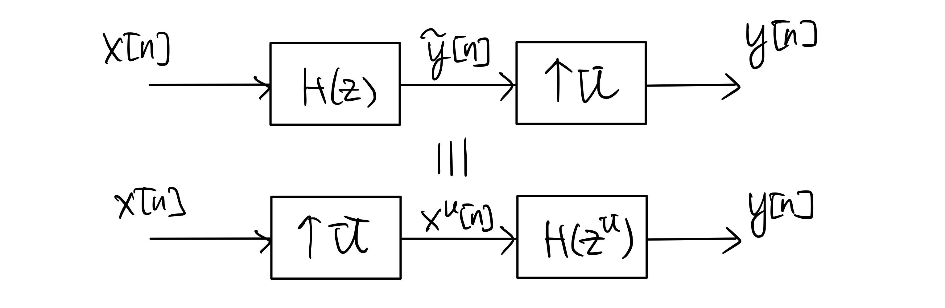
• We call the equivalence above the upsampling identity. To show this identity, recall from (7.3) that \(X^U(z) = X(z^U)\) in the second system. Similarly, considering the first system, we have

  \[\begin{align*} Y(z) &= \tilde{Y}(z^U) \\ &= H(z^U) X(z^U) \\ & = H(z^U) X^U(z) \end{align*}\]

  which is exactly the output of the second system; thus establishing the identity.

7.5.4. Downsample-DeMux Identity

• The following two systems are equivalent:

  

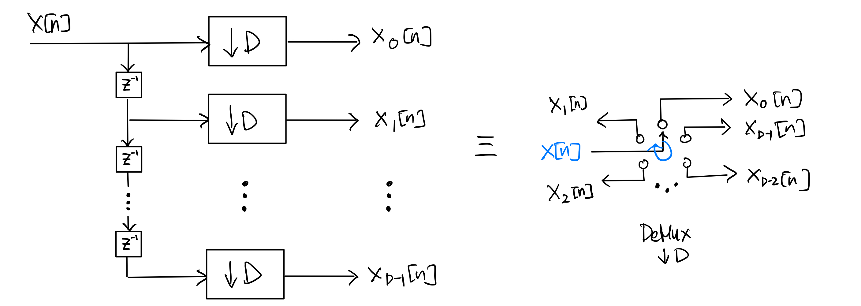
• The identity follows trivially by observing the system on the left that for \(k=0,1,\ldots, D-1\), \(x_k[n] = x_D[n-k] = x[nD-k]\), which is clearly the outputs of the demultiplexer on the right.

7.5.5. Upsample-Mux Identity

• The following two systems are equivalent:

  

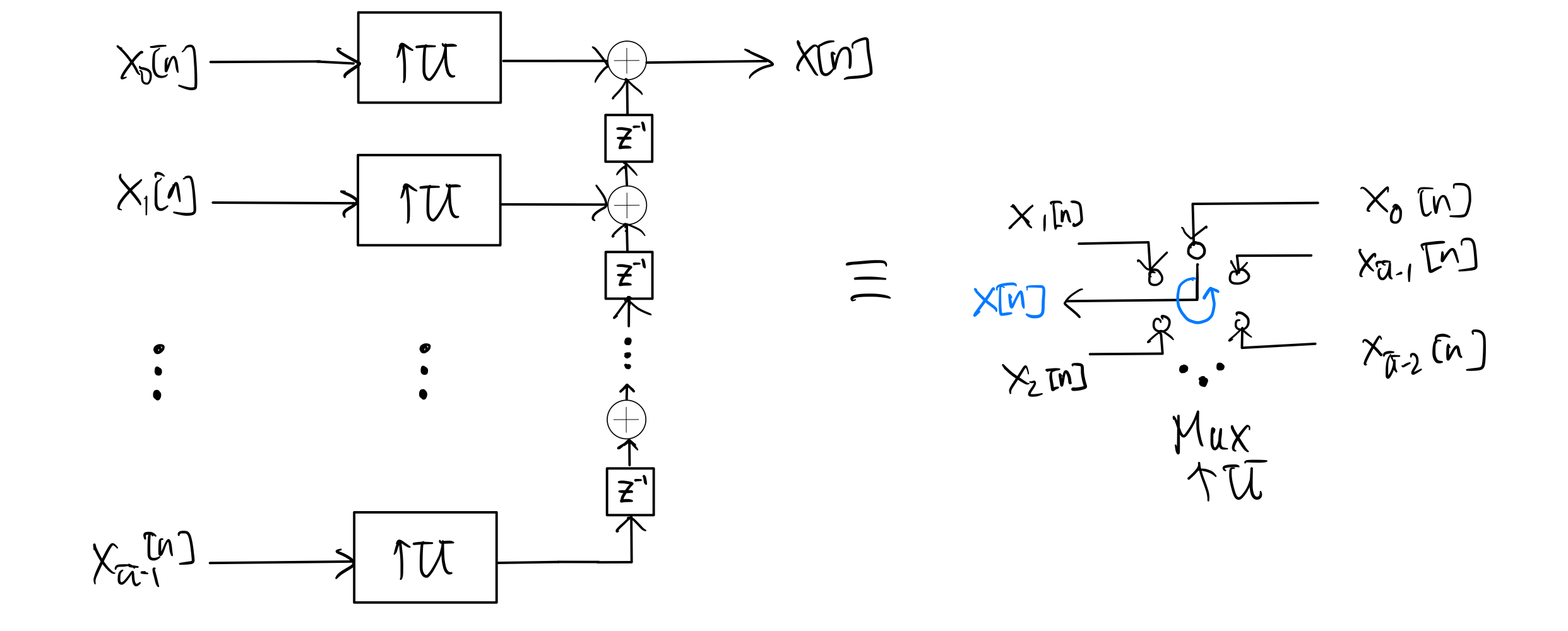
• The identity follows by observing the system on the left that

  \[\begin{equation*} x[n] = \sum_{l=0}^{U-1} x^U_l[n-l] \end{equation*}\]

  where \(x^U_l[n]\) is the upsampled signal by factor \(U\) from \(x_l[n]\), for \(l=0,1,\ldots, U-1\). Thus, for \(k=0,1,\ldots, U-1\),

  \[\begin{align*} x[nU+k] &= \sum_{l=0}^{U-1} x^U_l[nU+k-l] \\ &= x_k[n] \end{align*}\]

  because \(x^U_l[nU+k-l] = 0\) for \(k \neq l\). The fact that the signals \(x[nU+k]\), for \(k=0,1,\ldots, U-1\), are exactly the inputs to the multiplexer in the system on the right gives the identity.

7.5.6. Upsample-Downsample-Mux Identity

• The following two systems are equivalent:

  

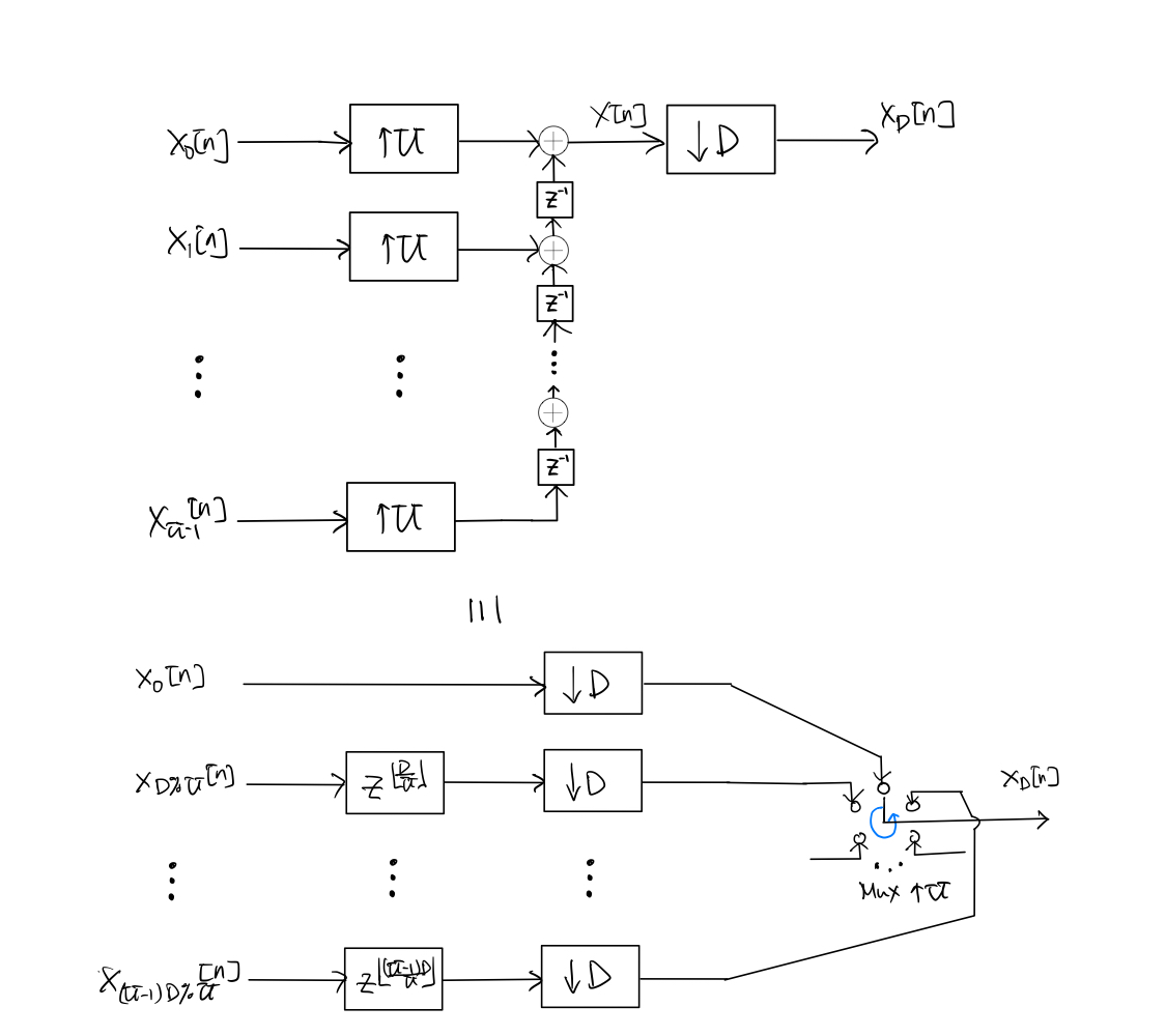
  where \(kD\%U = kD \bmod U\), i.e., the remainder of \(kD\) divided by \(U\).

• The identity follows by observing the system on the top that

  \[\begin{equation*} x[n] = \sum_{l=0}^{U-1} x^U_l[n-l]. \end{equation*}\]

  Thus, for \(k=0,1,\ldots, U-1\),

  (7.9)\[\begin{split}\begin{align} x_D[n] &= x[(nU+k)D] \\ &= \sum_{l=0}^{U-1} x^U_l[nUD+kD-l] \\ &= x^U_{kD\%U}[nUD+kD- (kD\%U)] \\ &= x^U_{kD\%U} \left[ \left(nD+\left\lfloor \frac{kD}{U} \right\rfloor \right)U \right] \\ &= x_{kD\%U} \left[ nD+\left\lfloor \frac{kD}{U} \right\rfloor \right] \end{align}\end{split}\]

  where the third equality is due to the fact that \(x^U_l[nUD+kD-l] = 0\) for \(l \neq kD\%U\), and the fourth equality is due to that fact that \(kD - (kD\%U) = \left\lfloor \frac{kD}{U} \right\rfloor U\). Note that signal \(x_{kD\%U} \left[ nD+\left\lfloor \frac{kD}{U} \right\rfloor \right]\) is simply the downsampled by \(D\) version of \(x_{kD\%U} \left[n + \left\lfloor \frac{kD}{U} \right\rfloor \right]\). Hence, (7.9) simply describes the operation of the system on the bottom of the figure above.