Polyphase Implementation of \frac{U}{D}-rate Filter

7.8. Polyphase Implementation of $\frac{U}{D}$-rate Filter#

Consider the general $\frac{U}{D}$-rate system as shown below with an LTI filter

$General $\frac{U}{D}$-rate filter$

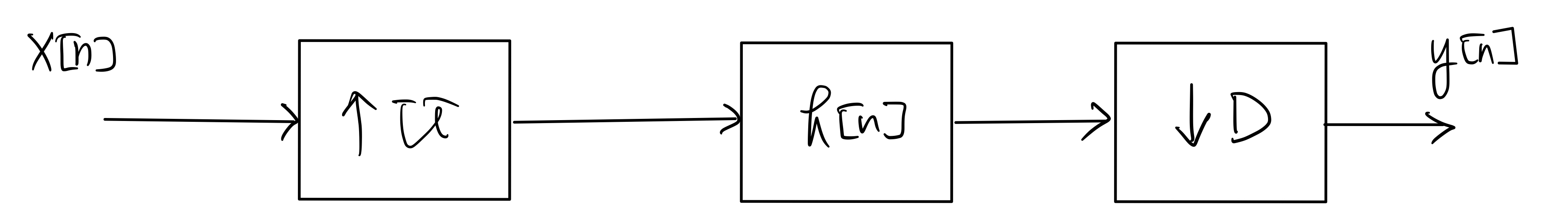
whose impulse response is $h[n] \stackrel{z}{\longleftrightarrow} H(z)$:

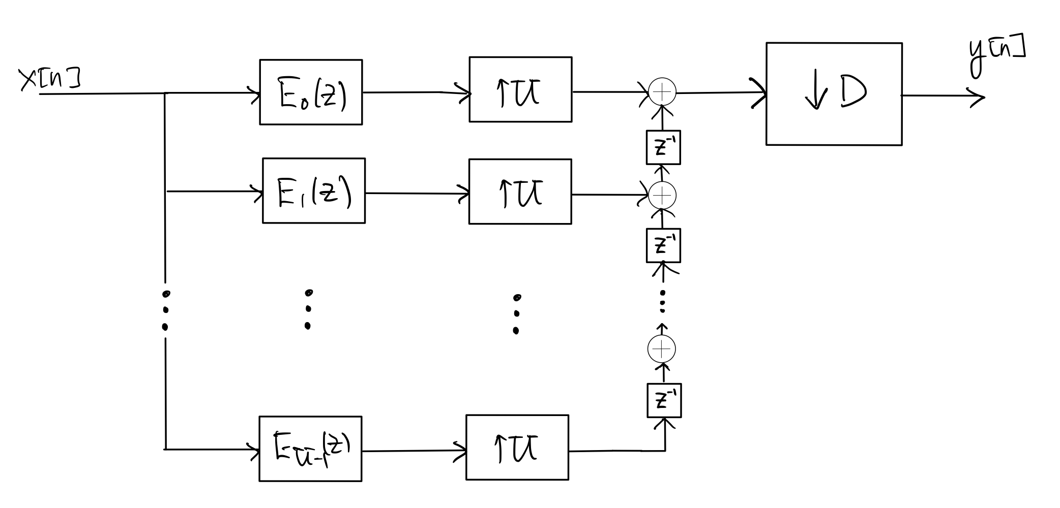
As in Section 7.7, applying the transposed form of the polyphase decomposition identity to $H(z)$ with $e_k[n] = h[nU+k]$, for $k=0,1,\ldots, U-1$, and then the upsampling identity to each branch gives

Next, applying the upsample-downsample-mux identity to the bank of upsamplers and the downsampler in step 1 gives
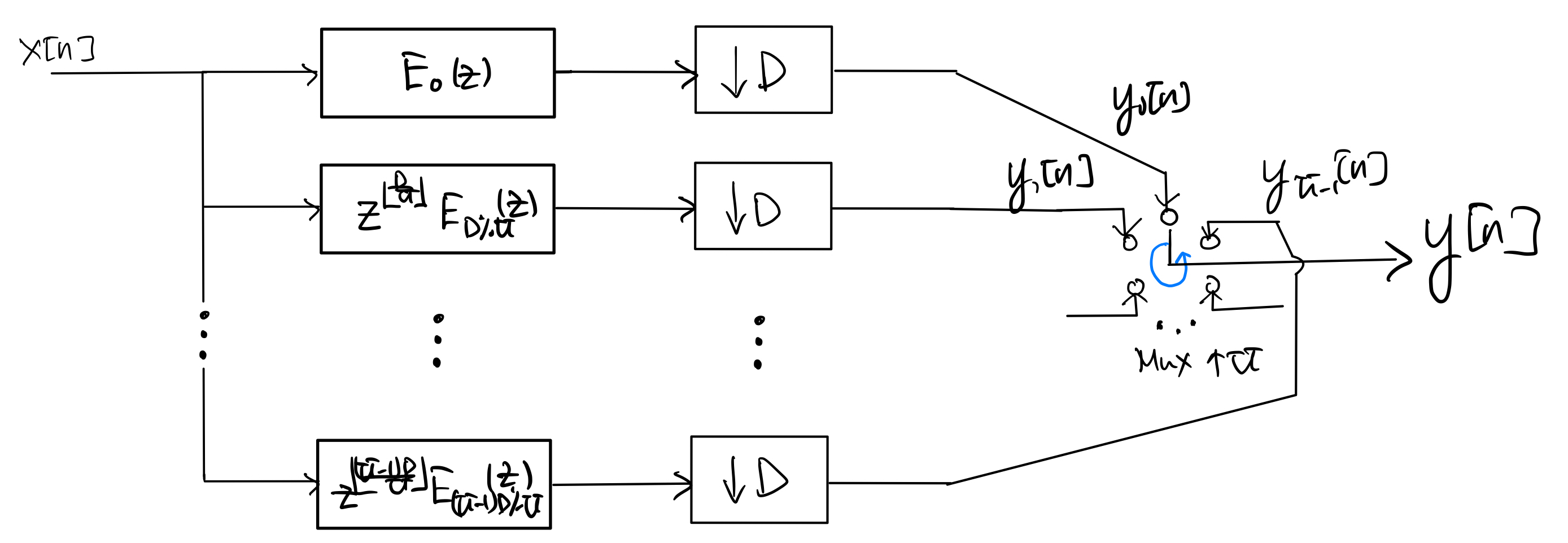
Then, for each $k=0,1,\ldots, U-1$, , as in Section 7.6, applying the direct form of the polyphase decomposition identity, downsampling identity, and downsample-demux identity to the $k$th branch in step 2 gives

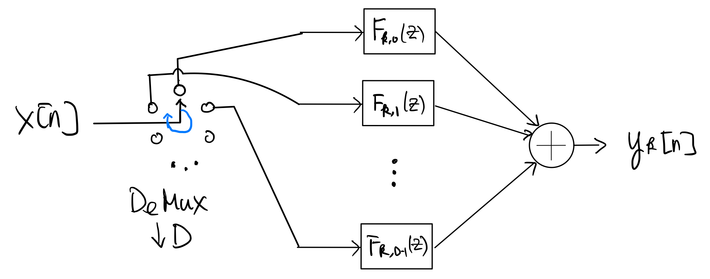
where the impulse response of the polyphase filter component $F_{k,l}$ is given by

\[\begin{align*} f_{k,l}[n] &= e_{kD\%U} \left[nD + \left\lfloor \frac{kD}{U} \right\rfloor + l \right] \\ &= h \left[ \left(nD + \left\lfloor \frac{kD}{U} \right\rfloor + l \right) U + kD\%U \right] \\ &= h[nUD + kD + lU] \end{align*}\]

for $l=0,1,\ldots, D-1$.

Caution

Note that some of the polyphase filter components $f_{l,k}[n]$ may be non-causal even if $h[n]$ is causal.
Finally, putting the polyphase implementation of the $k$th branch in step 3 back to the structure in step 2 gives the following overall polyphase implementation of the $\frac{U}{D}$-rate filter:

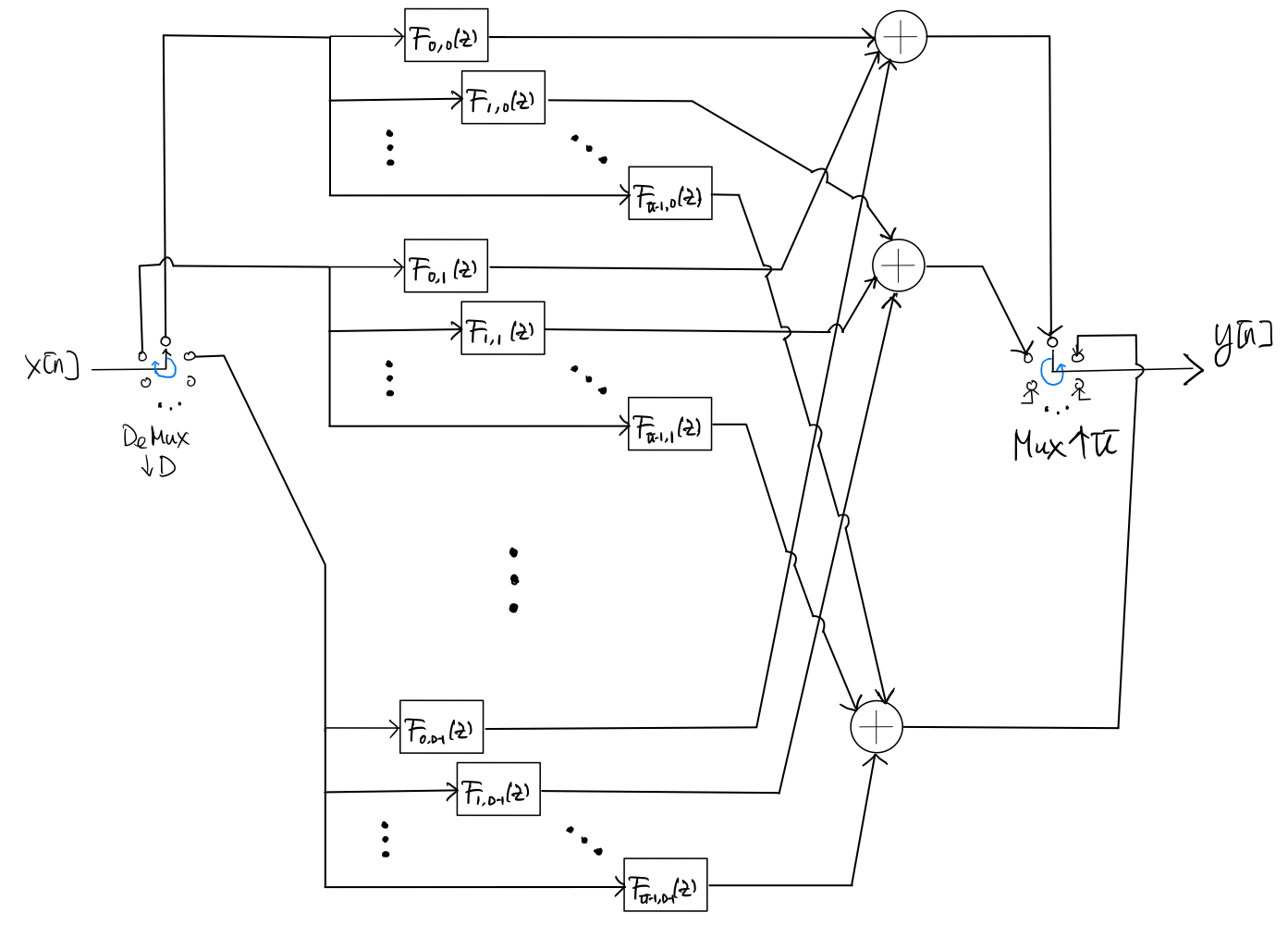
Note that all the polyphase component filters $F_{k,l}(z)$, $k=0,1,\ldots, U-1$ and $l=0,1,\ldots, D-1$, operate at $\frac{1}{D}$ times of the input rate. If $H(z)$ is an FIR filter of length $L$, then the length of $f_{k,l}[n]$ is at most $\lceil \frac{L}{UD} \rceil + 1$.
Clearly, the polyphase structure allows simple parallel implementation of the polyphase componet filters. Assuming $NU \gg L \gg UD$ where $N$ is the length of the input signal, the computational complexity (number of multiplications) of the polyphase implementation is $\mathcal{O}(\frac{L}{D})$ per input sample, instead of $\mathcal{O}(\frac{UL}{D})$ per input sample for the direct implementation.
The MATLAB functionupfirdn considered in the MATLAB example in Section 7.4 implements the polyphase structure in step 4 above.