5.4. Linear Filtering with FFT#
Consider passing a signal \(x[n]\) of length \(N\) to an FIR Filter with impulse response \(h[n]\) of length \(L\). In practice, we often have \(N \gg L \gg 1\). We will adopt this assumption in the discussion below.
Direct implementation of the convolution \(y[n] = h[n]*x[n]\) requires \(\mathcal{O}(NL)\) complex multiplications (and additions). While performing the filtering operation in the frequency domain using FFT algorithms to calculate DFT and IDFT as suggested in Section 5.2.3 requires \(\mathcal{O}(M\log_2 M)\) complex multiplications, where \(M \geq N+L-1\). Since \(N \gg L\), the computational complexity of this frequency-domain filtering approach is thus \(\mathcal{O}(N\log_2 N)\). Hence, if \(L \gg \log_2 N\), then we may obtain a significant reduction in computational complexity by performing frequency-domain filtering using FFT.
Nevertheless, the FFT implementation requires \(\mathcal{O}(N\log_2 N)\) complex storage units, as compared to the \(\mathcal{O}(N)\) required for direct convolution. The additional amount of storage requirement may be excessive if \(N\) is very large for say some embedded systems which may have limited amount of memory.
More importantly, frequency-domain filtering using FFT is a block processing approach. That is, one can not produce any output until the whole block of \(N\) input samples becomes available. This introduces a large latency in the filtering processing if \(N\) is large; thus preventing the applicability of the frequency-domain filtering approach in scenarios where real-time, low-latency processing is required.
5.4.1. Overlap-Add Algorithm#
The standard solution to the storage and latency problems is to:
break the long \(x[n]\) into consecutive smaller blocks of length \(\tilde{N}\),
perform frequency-domain filtering on each smaller block of length \(\tilde{N}\) with an FFT of a smaller (\(< N\)) size \(\tilde{M}\), and
combine the filter output blocks to obtain the output to the whole \(x[n]\).
To filter each smaller input block of length \(\tilde{N}\), one may choose the FFT size \(\tilde{M}\) satisfying \(\tilde{M} \geq \tilde{N} + L -1\) so that the output block contains the valid convolution result of length \(\tilde{N} + L -1\). The filtered output to the whole \(x[n]\) can then be obtained by superimposing overlapped blocks of output corresponding to consecutive blocks of input as shown in the diagram below:
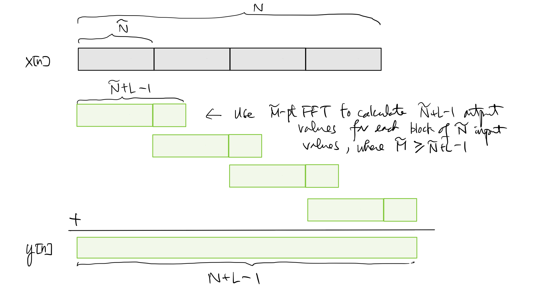
This approach to perform frequency-domain filtering is often referred to as the overlap-add algorithm.
Since we need to perform filtering on \(\frac{N}{\tilde{N}}\) input blocks and each block requires \(\mathcal{O}(\tilde{M} \log_2 \tilde{M})\) calculations, the computational complexity of filtering the whole input signal is this \(\mathcal{O}\left( \frac{N\tilde{M}}{\tilde{N}} \log_2 \tilde{M} \right)\) and the storage requirement is \(\tilde{M} \log_2 \tilde{M}\). For instance, if we choose \(\tilde{N} \sim L\) and \(\tilde{M} = \tilde{N}+L-1\), then the computational complexity becomes \(\mathcal{O}(N\log_2 L)\) and the storage requirement becomes \(\mathcal{O}(N+ L\log_2 L)\). Comparing with direct convolution, we can still get a significant reduction in computational complexity as long as \(L \gg 1\). The storage requirement is significantly lowered, compared with applying frequency-domain filtering with a single large-size FFT on the whole \(x[n]\). The filter latency reduces to \(\mathcal{O}(L)\).
5.4.2. Overlap-Save Algorithm#
Another approach is to:
break the long \(x[n]\) into consecutive overlapping blocks of length \(\tilde{M} \geq L\),
perform frequency-domain filtering on each input block of length \(\tilde{M}\) with an FFT of size \(\tilde{M}\), and
combine the filter output blocks to obtain the output to the whole \(x[n]\).
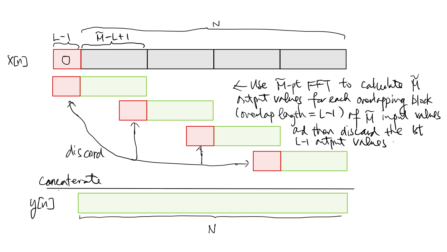
Since the length of the input block is the same as the FFT size, the frequency-domain filtering output gives us the circular convolution \((h \circledast_{\tilde{M}} x)[n]\) rather than the convolution \((h*x)[n]\) in this case. Referring back to (5.4), \((h\circledast_{\tilde{M}} x)[n]\) is the simply the periodic extension of \((h*x)[n]\), whose length is \(\tilde{M}+L-1\). Thus, it is easy to check that the last \(\tilde{M}-L+1\) samples in \((h\circledast_{\tilde{M}} x)[n]\) are not corrupted by time aliasing in the periodic extension process. That is, we have \((h\circledast_{\tilde{M}} x)[n] = (h*x)[n]\) for \(n=L-1, L, \ldots, \tilde{M}-1\). As a result, we may still be able to obtain the convolution output \(y[n]\) to the whole \(x[n]\) by concatenating the uncorrupted portions of the circular convoluted output blocks as long as the input blocks overlap by \(L-1\) samples. This leads to the overlap-save algorithm as depicted below:
It is also easy to check that the same orders of computational complexity, storage requirement, and latency of the overlap-add algorithm can be achieved by the overlap-save algorithm as well.