Multi-rate Filtering

7.4. Multi-rate Filtering#

A multi-rate filter is one whose input and output rates differ. That is, the filter outputs more/fewer than one sample per each input sample.
In practice, a fixed-rate ADC (and/or DAC) is often used. We may want to process the sampled signal at a rate different from the sampling rate of the ADC. In such cases, performing rate conversion in discrete time using a multi-rate filter would be convenient.
A general $\frac{U}{D}$-rate filter can be obtained by replacing the ideal lowpass filter in the rate conversion system in Section 7.3 with a general lowpass filter $h[n]$ operating at the interpolated rate $U$:
$$\frac{U}{D}$-rate filter$
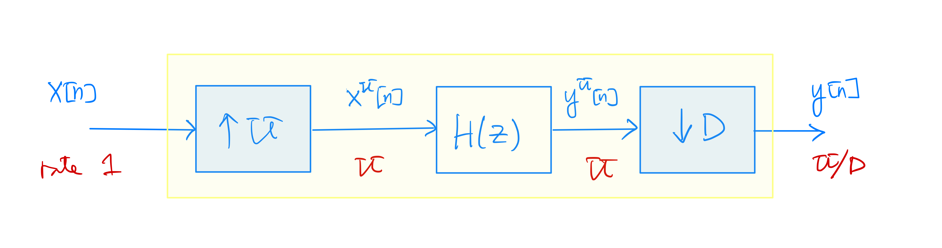
Clearly, if $X(e^{j\hat\omega}) \neq 0$ for $\frac{U\pi}{D} \leq |\hat\omega| \leq \pi$, we must have $H(e^{j\hat\omega}) = 0$ for $\frac{\pi}{\max(U,D)} \leq |\hat\omega| \leq \pi$ for interpolation and anti-aliasing.
Direct implementation of the multi-rate filter above may not be desirable in practice because the filter $h[n]$ needs to be implemented at $U$ times the input rate.
For the case that $h[n]$ is an FIR filter of length $L$, a direct time-domain implementation (convolution) of the $\frac{U}{D}$-rate filter requires $\displaystyle \left\lfloor \frac{NU+L-1}{D} \right\rfloor L$ multiplications when the length of the input signal is $N$. Assuming $NU \gg L \gg UD$, the number of multiplications needed to implement the $\frac{U}{D}$-rate is thus $\mathcal{O}(\frac{UL}{D})$ per input sample.
One may reduce the computational complexity of implementing the $\frac{U}{D}$-rate filter by performing frequency-domain filter using FFT based on the overlap-save or overlap-add algorithm discussed in Section 5.4.
MATLAB Example:

In this example, we design and implement a $\frac{3}{2}$-rate FIR filter to convert a chirp signal that is sampled at $500$ samples per second to one that is sampled $750$ samples per second. The chirp signal is specified by $x(t) = \cos(800\pi t^2)$. First, generate the sampled version of the chirp at $f_s=500$ for a duration of $0.1$ seconds:
```
>> fs = 500;
>> t = 0:1/fs:0.1;
>> x = cos(800*pi*t.*t);
```
From Section 7.3, we need to design a lowpass FIR filter with cutoff at $\frac{\pi}{3}$ and passband magnitude $3$ to work as the interpolation filter. Here, we pick the specification $(\frac{\pi}{3}, 0.35\pi, 0.01, 0.01)$ and use the Parks-McClellan algorithm to obtain a generalized linear-phase FIR filter:
```
>> [M, we, A, W] = firpmord([1/3, 0.35], [3, 0], [0.01, 0.01])


M =

   272

we =

         0
    0.3333
    0.3500
    1.0000

A =

     3
     3
     0
     0

W =

     3
     1

>> h = firpm(M, we, A, W);
>> fvtool(h, 1);
```
With the interpolation filter designed, we can then use the MATLAB function upfirdn to implement the rate conversion:
```
>> y = upfirdn(x, h, 3, 2);
```
We may plot the original sampled signal x and the rate-converted signal y together on the same figure to see the equivalent effect of increasing the sampling rate to $750$ samples per second:
```
>> stem(((0:length(y)-1)*2-M/2)/3/fs, y, 'rx')
>> hold on;
>> stem((0:length(x)-1)/fs, x, 'bo');
>> tt = 0:1/fs/100:0.1;
>> xx = cos(800*pi*tt.*tt); 
>> plot(tt, xx, 'k'); %plot continuous-time chirp
```
Caution

Recall that the generalized linear-phase filter has a group delay of $\frac{M}{2} = 136$ samples at the interpolated rate. Thus, we need to left-shift the rate-converted signal y in the figure to make it align with the original sampled signal x for comparison.