3.2. Sampling Theorem#
Suppose that a continuous-time signal \(x(t)\) is sampled at the sampling rate of \(f_s\) samples per second to obtain the discrete-time signal \(x[n] = x(\frac{n}{f_s})\). The frequency-domain version of the Poisson sum formula (3.5) relates the DTFT \(X(e^{j\hat\omega})\) of the sampled signal \(x[n]\) to the FT \(X(\omega)\) of the original continuous-time signal \(x(t)\):
(3.6)#\[\begin{equation} X(e^{j\hat\omega}) = f_s \sum_{k=-\infty}^{\infty} X((\hat\omega+2\pi k)f_s) \end{equation}\]where the quantity on the RHS is often referred to as the folded spectrum of \(x(t)\). In other words, the DTFT of the sampled signal \(x[n]\) is the folded spectrum of \(x(t)\).
Tip
One may extend the Poisson sum formula to include all finite-energy and some common infinite-energy signals and FTs based on the limiting process with windowing as we did before.
From (3.6), it is clear that the folded spectrum depends on both the FT of the continuous-time signal and the sampling rate. The effects of both factors are best explained in picture. First, let us introduce the concept of bandlimtedness:
Notation
A continuous-time signal \(x(t)\) is bandlimited to \(\Omega = 2\pi B\) radian per second (or \(B\) Hz) if its FT \(X(\omega) = 0\) for \(|\omega| > \Omega\). The quantity \(\Omega\) (or \(B\)) is called the bandwidth of \(x(t)\).
For a simple illustration, consider a bandlimited continuous-time signal \(x(t)\) whose FT \(X(\omega)\) is of real-valued and as shown below:
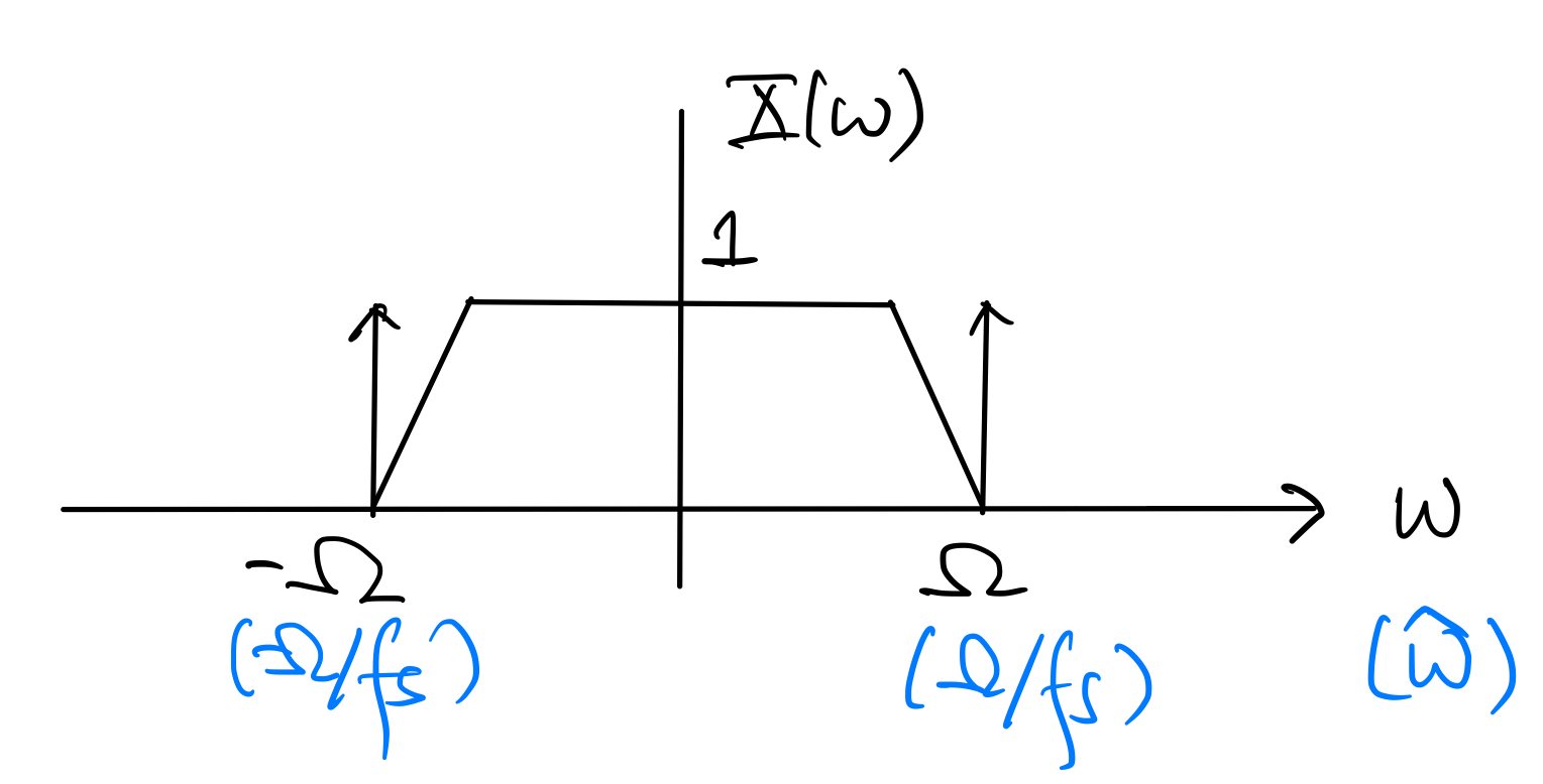
The bandwidth of \(x(t)\) is \(\Omega\) radians per second, or \(B\) Hz. To draw the folded spectrum of \(x(t)\), we need to consider two different cases:
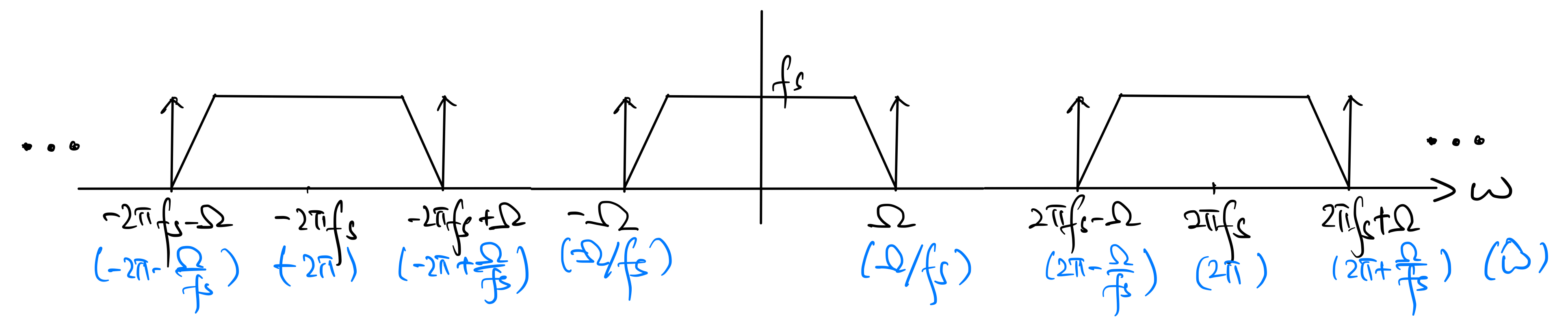
If \(f_s > 2B\), then the folded spectrum is as below:
Notation
The condition \(f_s > 2B\) is referred to as oversampling. The sampling rate \(2B\) is usually referred to as the Nyquits rate.
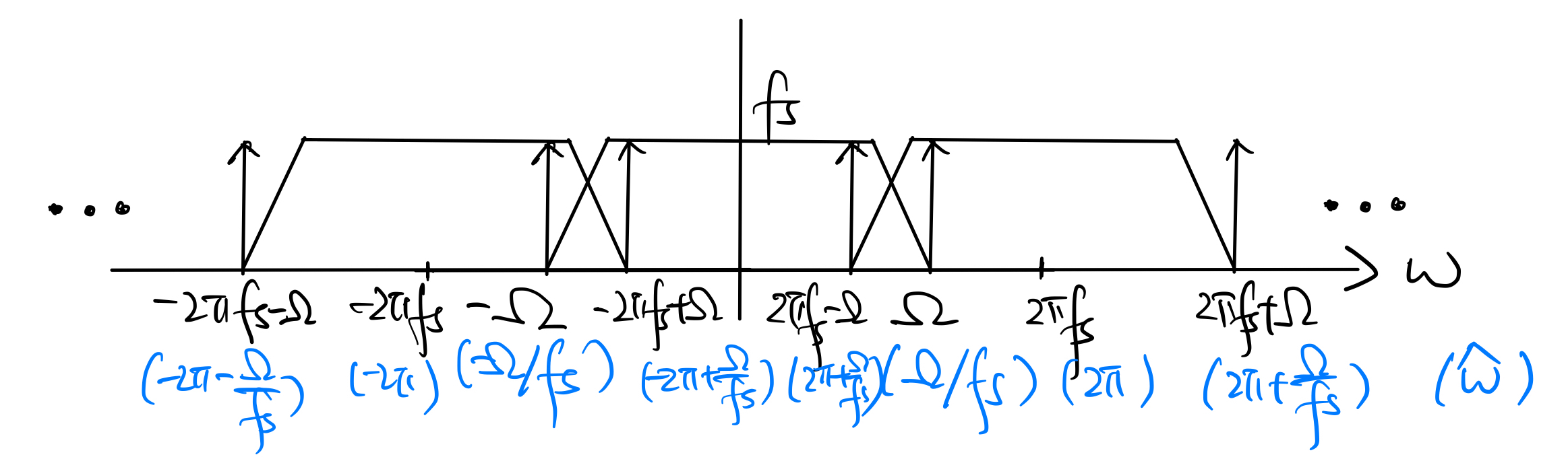
If \(f_s \leq 2B\), then the folded spectrum is as below:
Notation
The condition \(f_s \leq 2B\) is referred to as undersampling.
3.2.1. Oversampling (\(f_s > 2B\))#
In this case, we can see from the plot that the FT \(X(\omega)\) of the original continuous-time signal is perserved in the folded spectrum \(X(e^{j\hat\omega})\). Thus, \(X(\omega)\) can be easily recovered from \(X(\omega)\), or equivalently in the time domain, \(x(t)\) can be recovered from \(x[n]\).
In the frequency domain, the ideal reconstruction process is simply:
Cut out the period of the folded spectrum \(X(e^{j\hat\omega})\) over \([-\pi, \pi)\) and scale it by \(\frac{1}{f_s}\).
Substitute \(\hat\omega = \frac{\omega}{f_s}\) in the cut-out and scaled period of \(X(e^{j\hat\omega})\) to convert it to the FT \(\tilde{X}(\omega)\) of the reconstructed continuous-time signal \(\tilde{x}(t)\), i.e.,
(3.7)#\[\begin{split} \begin{equation} \tilde{X}(\omega) = \begin{cases} \frac{1}{f_s} X\left( e^{j\frac{\omega}{f_s}} \right), & \text{if } -\pi f_s < \omega < \pi f_s \\ 0, & \text{otherwise.} \end{cases} \end{equation}\end{split}\]Since \(X(\omega) = 0\) for \(|\omega| > \Omega\) (\(x(t)\) is bandlimited to \(\Omega\)) and \(\pi f_s > \Omega\), we have \(\tilde{X}(\omega) = X(\omega)\), which of course implies \(\tilde{x}(t) = x(t)\) in the time domain.
Let us reconsider the ideal reconstruction steps above from a time-domain perspective:
(3.8)#\[\begin{split}\begin{align} \tilde{x}(t) &= \frac{1}{2\pi} \int_{-\infty}^{\infty} \tilde{X}(\omega) e^{j\omega t} \, d\omega \\ &= \frac{1}{2\pi} \int_{-\pi f_s}^{\pi f_s} \frac{1}{f_s} X\left( e^{j\frac{\omega}{f_s}} \right) e^{j\omega t} \, d\omega \\ &= \frac{1}{2\pi} \int_{-\pi f_s}^{\pi f_s} \left( \frac{1}{f_s} \sum_{n=-\infty}^{\infty} x[n] e^{-j\frac{\omega n}{f_s}} \right) e^{j\omega t} \, d\omega \\ &= \sum_{n=-\infty}^{\infty} x[n] \frac{1}{2\pi} \int_{-\pi f_s}^{\pi f_s} \frac{1}{f_s} e^{j\omega \left( t - \frac{n}{f_s} \right)} \, d\omega \\ &= \sum_{n=-\infty}^{\infty} x[n] \cdot \frac{\sin\left( \pi f_s (t-\frac{n}{f_s}) \right)}{ \pi f_s (t-\frac{n}{f_s})} \end{align}\end{split}\]Since \(\tilde{x}(t)=x(t)\) if \(\pi f_s > \Omega\), we obtain the following result which is usually referred to as the sampling theorem:
Sampling Theorem
Consider sampling a continuous-time signal \(x(t)\) that is bandlimited to \(B\) Hz at the sampling rate of \(f_s\) samples per second to obtain the discrete-time signal \(x[n] = x(\frac{n}{f_s})\). If \(f_s > 2B\), then
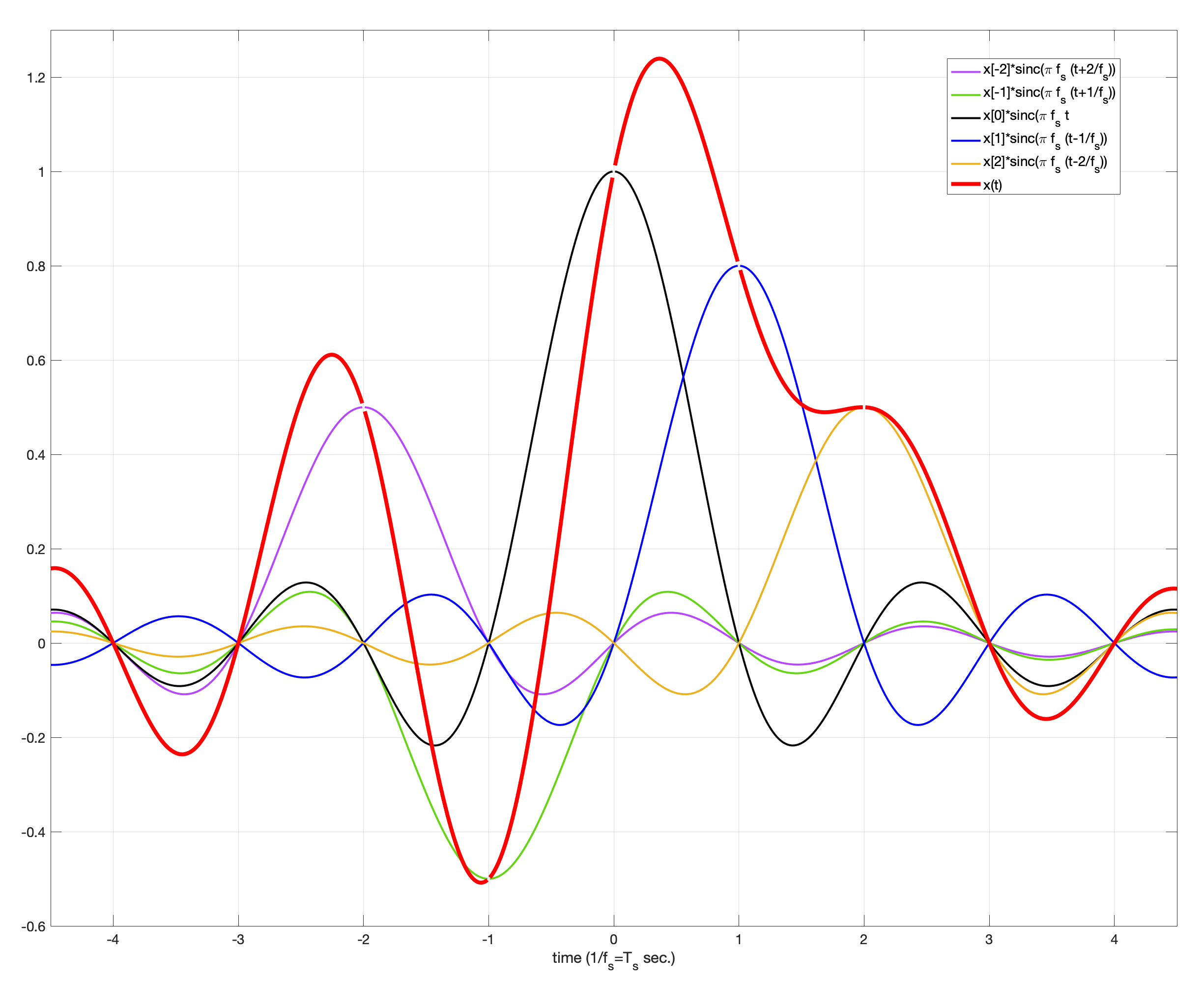
(3.9)#\[\begin{equation} x(t) = \sum_{n=-\infty}^{\infty} x[n] \, \text{sinc} \left( \pi f_s (t-\frac{n}{f_s}) \right) \end{equation}\]where \(\text{sinc}(t) = \frac{\sin t}{t}\).
To illustrate the sampling theorem in picture, let us first plot the sinc kernel (signal) \(\text{sinc}(\pi f_s t)\):
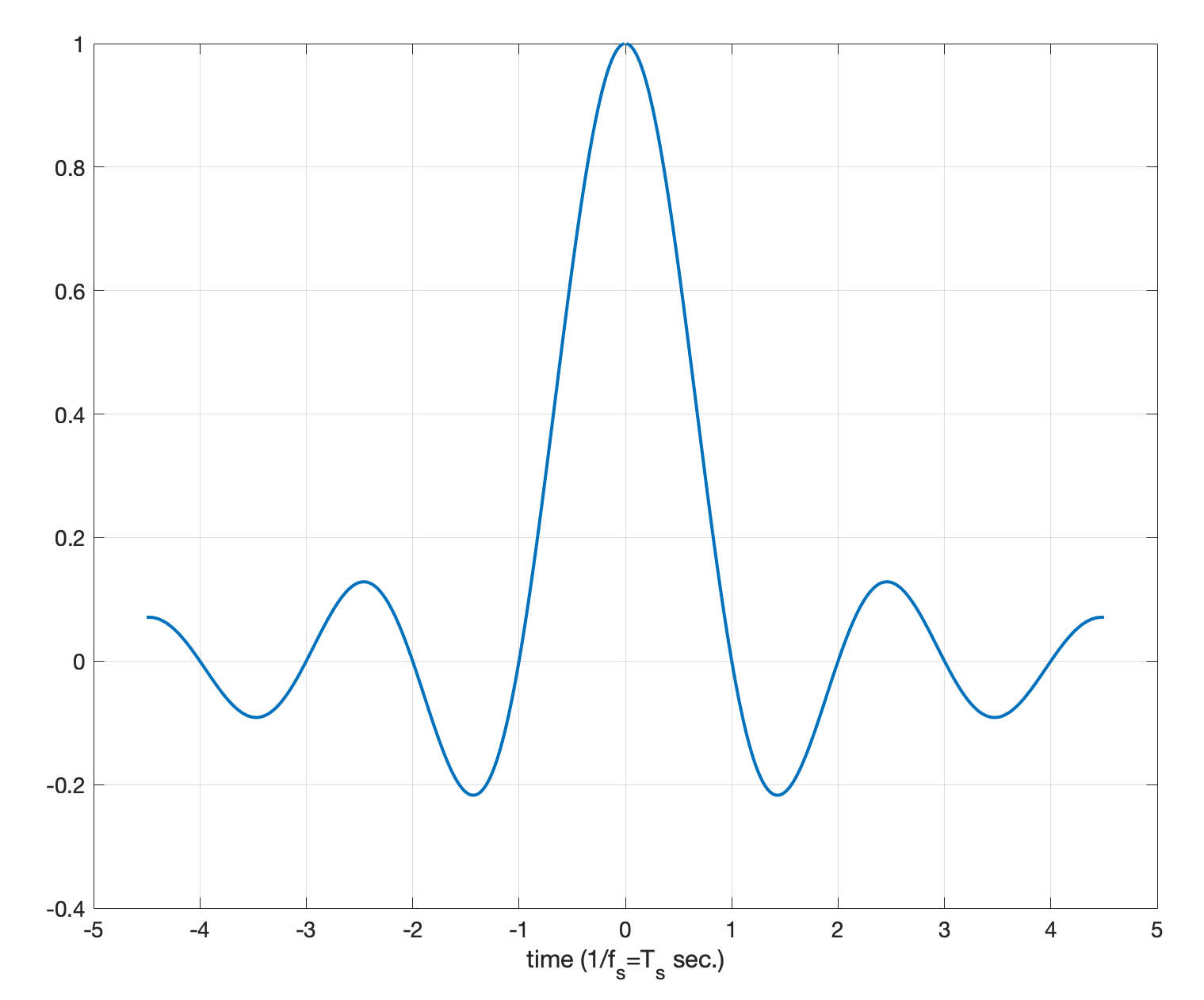
The sampling theorem says that the original continuous-time signal \(x(t)\) can be reconstructed by interpolating the discrete-time (sampled) signal \(x[n]\) using the sinc kernel as long as we oversample:
In practice, we can’t use the ideal sinc kernel to perform interpolation because the length (support) of the sinc kernel is infinite. We have to approximate the reconstruction by using a truncated version of the sinc kernel or other kernels of finite support:
zero-order hold: rectangular kernel \(\begin{cases} 1, & \text{if } |t| < \frac{1}{2f_s} \\ 0, & \text{otherwise.} \end{cases}\)
first-order hold (linear interpolation): triangular kernel \(\begin{cases} 1 - f_s |t|, & \text{if } |t| < \frac{1}{f_s} \\ 0, & \text{otherwise.} \end{cases}\)
A typical practical implementation employs zero-order hold interpolation and then passes the reconstructed signal through an analog lowpass filter to further smooth it. The combination of the zero-order hold interpolation and lowpass filtering is equivalent to using an interpolation kernel that is the convolution between the rectangular kernel and the impulse response of the lowpass filter.
3.2.2. Undersampling (\(f_s \leq 2B\))#
In this case, we see from the plot of the folded spectrum that the frequency-shifted copies of \(X(\omega)\) superimpose on each other. This phenomenon is usually called aliasing. Thus, \(X(\omega)\) cannot be recovered from the folded spectrum using the simple steps in the case of oversampling because \(\tilde{X}(\omega) \neq X(\omega)\).
Nevertheless, the interpolation formula in (3.8) is still valid, but \(\tilde{x}(t) \neq x(t)\). The reconstructed signal \(\tilde{x}(t)\) given by (3.8) is called the aliased version of \(x(t)\).
Caution
Note that undersampling \(x(t)\) doesn’t necessarily means that there is no possibility of recovering it from the sampled signal \(x[n]\). However, to be able to do so may require \(x(t)\) to have some special structures and more significant signal processing.
In practice, to avoid the “uncontrolled” effects of aliasing, the continuous-time signal \(x(t)\) is usually passed through an analog lowpass filter with cutoff frequency \(\frac{f_s}{2}\) Hz to remove any frequency components in \(x(t)\) that are above \(\frac{f_s}{2}\) Hz before sampling. The lowpassed signal then will not suffer from aliasing. The analog lowpass filter is often called an antialiasing filter. Of course, we may only reconstruct the lowpassed version of \(x(t)\) from the sampled signal. Nevertheless, applying the antialiasing filter allows us to control the distortion we may suffer from potential undersampling.
3.2.3. Nyquist Zone Sampling of Bandpass Signal#
In some situations, we may be able to turn the undesirable phenomenon of aliasing into an advantage. One such situation is the undersampling of a bandpass continuous-time signal.
First, we have to define what a bandpass continuous-time signal is:
Notation
A (real-valued) continuous-time signal \(x(t)\) is bandpass with a center frequency at \(\omega_0=2\pi f_0\) radian per second (or \(f_0\) Hz) and a bandwidth of \(\Omega = 2\pi B\) radian per second (or \(B\) Hz) if its FT \(X(\omega) = 0\) for \(|\omega| \notin [\omega_0 - \frac{\Omega}{2}, \omega_0 + \frac{\Omega}{2}]\).
Clearly, the Nyquist rate of the bandpass signal \(x(t)\) is \(2f_0+B\) Hz. We must sample \(x(t)\) at above \(2f_0+B\) sps to avoid aliasing. Nevertheless, sampling of the bandpass signal \(x(t)\) is a situation in which we may want to deliberately undersample in order to exploit aliasing to our advantage.
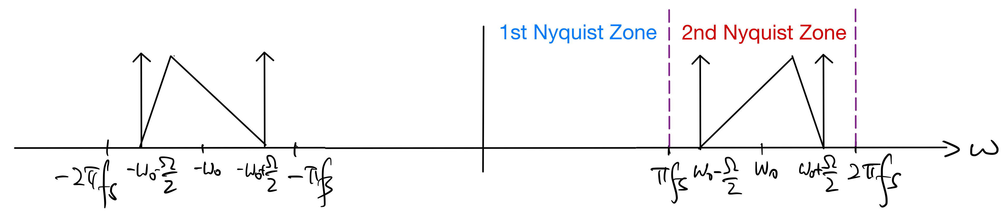
Consider undersampling \(x(t)\) with at the sampling rate \(f_s\) satisfying the condition \(f_0 + \frac{B}{2} < f_s < 2f_0 -B\). That is, all frequency components of \(x(t)\) lie within the frequency range \((\frac{f_s}{2}, f_s)\) Hz, which is often referred to as the second Nyquist zone. This is in reference to that the frequency range \([0, \frac{f_s}{2})\) Hz is called the first Nyquist zone. A pictorial illustration of a (real-valued) bandpass \(x(t)\) with its whole \(X(\omega)\) lying in the second Nyquist zone is as shown below:
Applying the folded spectrum formula (3.6) to obtain the DTFT \(X(e^{j\hat\omega})\) of the sampled signal \(x[n] = x(\frac{n}{f_s})\) gives the following folded spectrum:
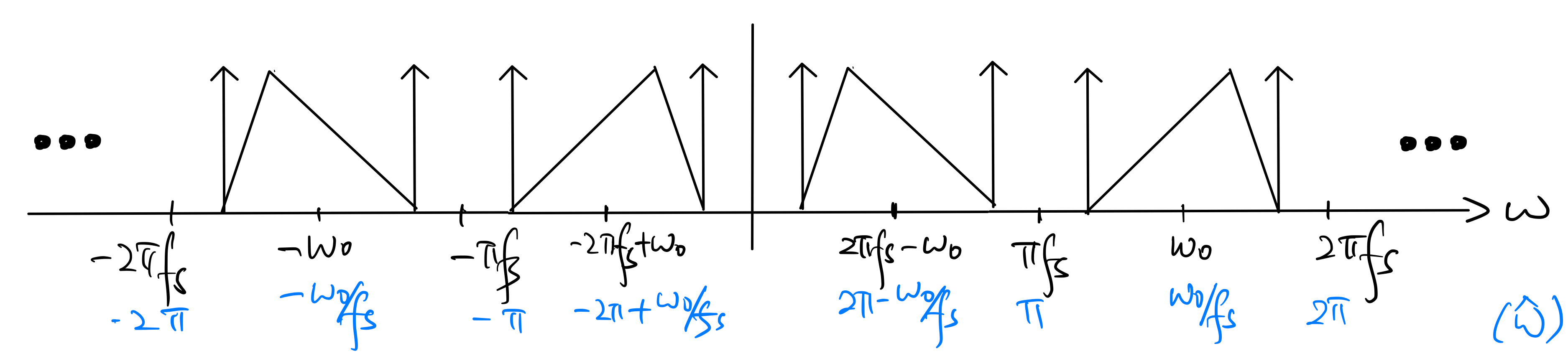
We see the all spectrum information in the FT \(X(\omega)\) of the original continuous-time \(x(t)\) is preserved in the folded spectrum \(X(e^{j\hat\omega})\) of the sampled signal \(x[n]\) in this case. That is, we may get back \(X(\omega)\) from \(X(e^{j\hat\omega})\) (equivalently \(x(t)\) from \(x[n]\)), although the reconstruction operation is a bit more complicated than that in the oversampling case as shown in Section 3.2.1 above.
Often, it is more convenient for subsequent processing to “bring” \(x[n]\) (which is a discrete-time bandpass signal itself) down to the baseband by passing its frequency-shifted version \(x[n] e^{j(2\pi - \frac{\omega_0}{f_s})n}\) through an ideal lowpass filter with cutoff frequency \(\frac{\Omega}{2f_s}\) radian per sample. The resulting signal will have the following DTFT:
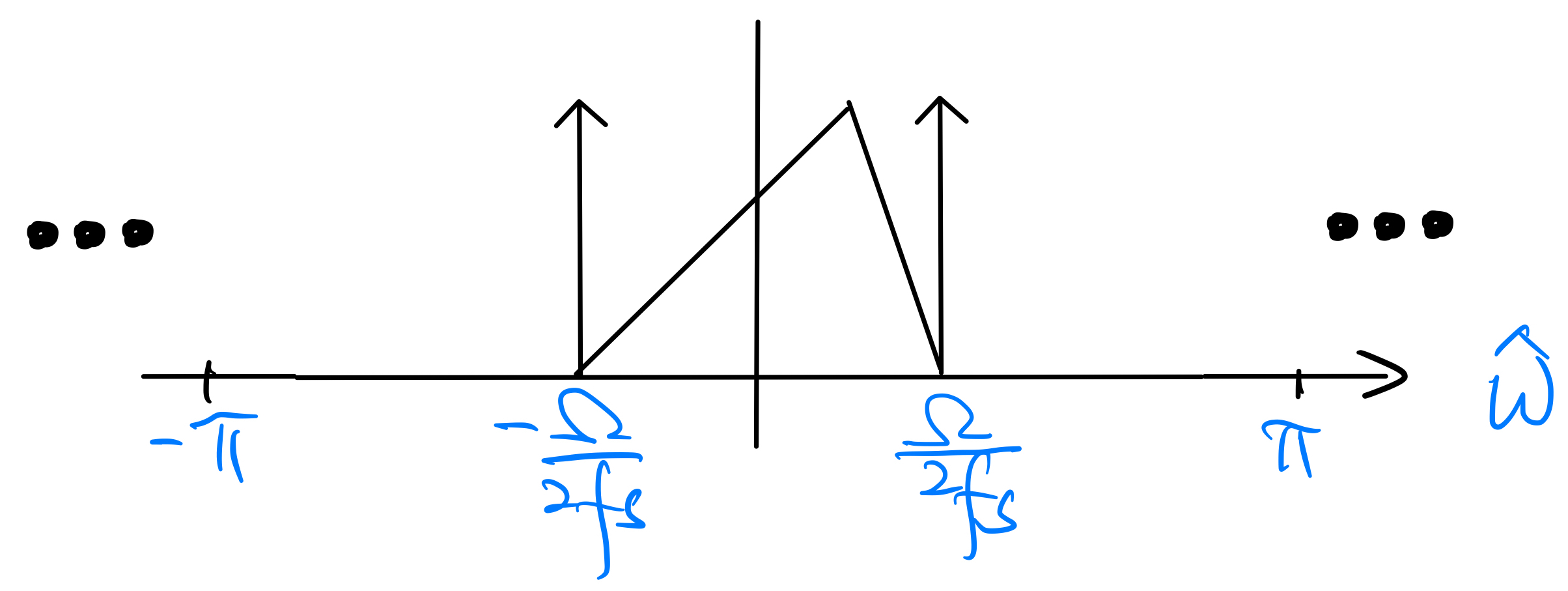
This signal at the output of the lowpass filter is often called the complex baseband version of \(x[n]\). It is a complex-valued bandlimited signal and retains all spectrum information of the original continuous-time \(x(t)\), i.e., we can reconstruct \(x(t)\) from this complex baseband signal.
In practice, we often pass the bandpass continuous-time signal \(x(t)\) through an analog bandpass filter with passband coinciding the second Nyquist zone to remove all its frequency components outside of the second Nyquist zone before sampling. This bandpass filter acts in the same way as the anti-aliasing filter as discussed in Section 3.2.2.
It is easy to see that the same aliasing trick theoretically applies to bandpass signals lying in any “higher” Nyquist zones. However, the sampling operation in practical ADCs is not ideal. The effect of non-ideal sampling may be thought of as first lowpass filtering the continuous-time bandpass signal and then performing ideal sampling. Hence, a bandpass signal lying in a high Nyquist zone may be attenuated (and perhaps also distorted) too much that the sampled version may suffer significantly from the quantization noise of the ADC. As a result, Nyquist zone sampling is often limited to the second or third Nyquist zone in practice.