7.1. Downsampling#
Given \(x[n] \stackrel{z}{\longleftrightarrow} X(z)\). Consider the downsampled signal \(x_D[n] = x[Dn]\), where \(D\) is a positive integer. That is, we obtain \(x_D[n]\) by sampling \(x[n]\) every \(D\) time instants:
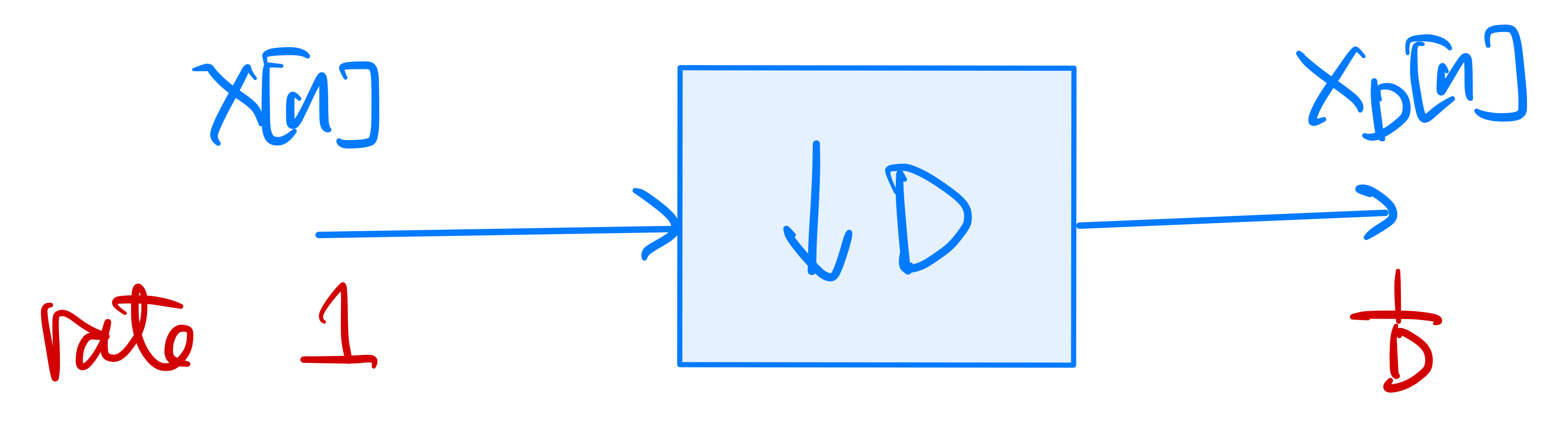
The rate of \(x_D[n]\) is \(\frac{1}{D}\) times that of \(x[n]\). That is, every \(D\) samples of \(x[n]\) gives \(1\) sample pf \(x_D[n]\).
Recall, from Section 2.4.3 and Section 2.4.4, the impulse train \(\displaystyle \delta_D[n] = \sum_{k=-\infty}^{\infty} \delta[n-kD]\) of period \(D\) and its DFS expansion \(\displaystyle \delta_D[n] = \frac{1}{D} \sum_{k=0}^{D-1} e^{j\frac{2\pi k n}{D}}\). Let \(\tilde{x}[n] = x[n] \delta_D[n] = \begin{cases} x[n] & \text{if } n \text{ is divisible by } D \\ 0 & \text{otherwise.} \end{cases}\)
Then, it is trivial to check that \(x_D[n] = \tilde{x}[Dn]\).
Consider the \(z\)-transform \(X_D(z)\) of the downsampled signal \(x_D[n]\):
(7.1)#\[\begin{split}\begin{align} X_D(z) &= \sum_{n=-\infty}^{\infty} x_D[n] z^{-n} \\ &= \sum_{n=-\infty}^{\infty} \tilde{x}[Dn] z^{-n} \\ &= \sum_{m=-\infty}^{\infty} \tilde{x}[m] z^{-\frac{m}{D}} \\ &= \sum_{m=-\infty}^{\infty} x[m] \delta_D[m] z^{-\frac{m}{D}} \\ &= \sum_{m=-\infty}^{\infty} x[m] \left( \frac{1}{D} \sum_{k=0}^{D-1} e^{j\frac{2\pi k m}{D}} \right) z^{-\frac{m}{D}} \\ &= \frac{1}{D} \sum_{k=0}^{D-1} \sum_{m=-\infty}^{\infty} x[m] \left( e^{-j\frac{2\pi k}{D}} z^{\frac{1}{D}} \right)^{-m} \\ &= \frac{1}{D} \sum_{k=0}^{D-1} X\left( e^{-j\frac{2\pi k}{D}} z^{\frac{1}{D}} \right). \end{align}\end{split}\]Tip
If \(x[n]\) is causal and the ROC of \(X(z)\) is \(\{|z| > r\}\), then the ROC of \(X_D(z)\) is \(X(z)\) is \(\{|z| > r^D\}\).
Suppose the ROC of \(X(z)\) contains the unit circle. Then the ROC of \(X_D(z)\) also does, and hence the DTFT of the downsampled signal \(x_D[n]\) is given by
(7.2)#\[\begin{equation} X_D(e^{j\hat\omega}) = \frac{1}{D} \sum_{k=0}^{D-1} X\left( e^{j \frac{\hat\omega - 2\pi k}{D}} \right) \end{equation}\]which looks like the Poisson sum formula (3.6) that gives rise to the folded spectrum of the discrete-time signal obtained from sampling a continuous-time one, except that only \(D\) frequency-shifted (and scaled) copies of \(X(e^{j\hat\omega})\) are superimposed with a sampling rate of \(\frac{1}{D}\).
In fact, if \(x[n]\) is obtained from sampling a continuous-time signal \(x(t) \stackrel{\text{FT}}{\longleftrightarrow} X(\omega)\) at sampling rate \(f_s\), then \(x_D[n]\) is clearly the sampled version of \(x(t)\) at sampling rate \(\frac{f_s}{D}\). In terms of the folded spectrum, \(\displaystyle X(e^{j\hat\omega}) = f_s \sum_{l=-\infty}^{\infty} X(\hat\omega f_s + 2\pi l f_s)\). Hence, by (7.2) we have
\[\begin{align*} X_D(e^{j\hat\omega}) &= \frac{1}{D} \sum_{k=0}^{D-1} f_s \sum_{l=-\infty}^{\infty} X\left( \frac{(\hat\omega -2\pi k + 2\pi l D) f_s}{D} \right) \\ &= \frac{f_s}{D} \sum_{l'=-\infty}^{\infty} X\left( \hat\omega \frac{f_s}{D} + 2\pi l' \frac{f_s}{D} \right) \end{align*}\]which is exactly the folded spectrum generated by sampling \(x(t)\) at sampling rate \(\frac{f_s}{D}\).
Similar to sampling a continuous-time signal, downsampling a discrete-time signal may also suffer from aliasing. Again, we need to consider two cases, depending on the DTFT \(X(e^{j\hat\omega})\), when examining the effect of the folded spectrum resulted from downsampling described by (7.2):
Oversampling \(X(e^{j\hat\omega}) = 0\) for \(\frac{\pi}{D} \leq |\hat\omega| \leq \pi\):
The folded spectrum \(X_D(e^{j\hat\omega D}) = \frac{1}{D} \sum_{k=0}^{D-1} X\left( e^{j (\hat\omega - \frac{2\pi k}{D})} \right)\) for this case is illustrated in the figure below:
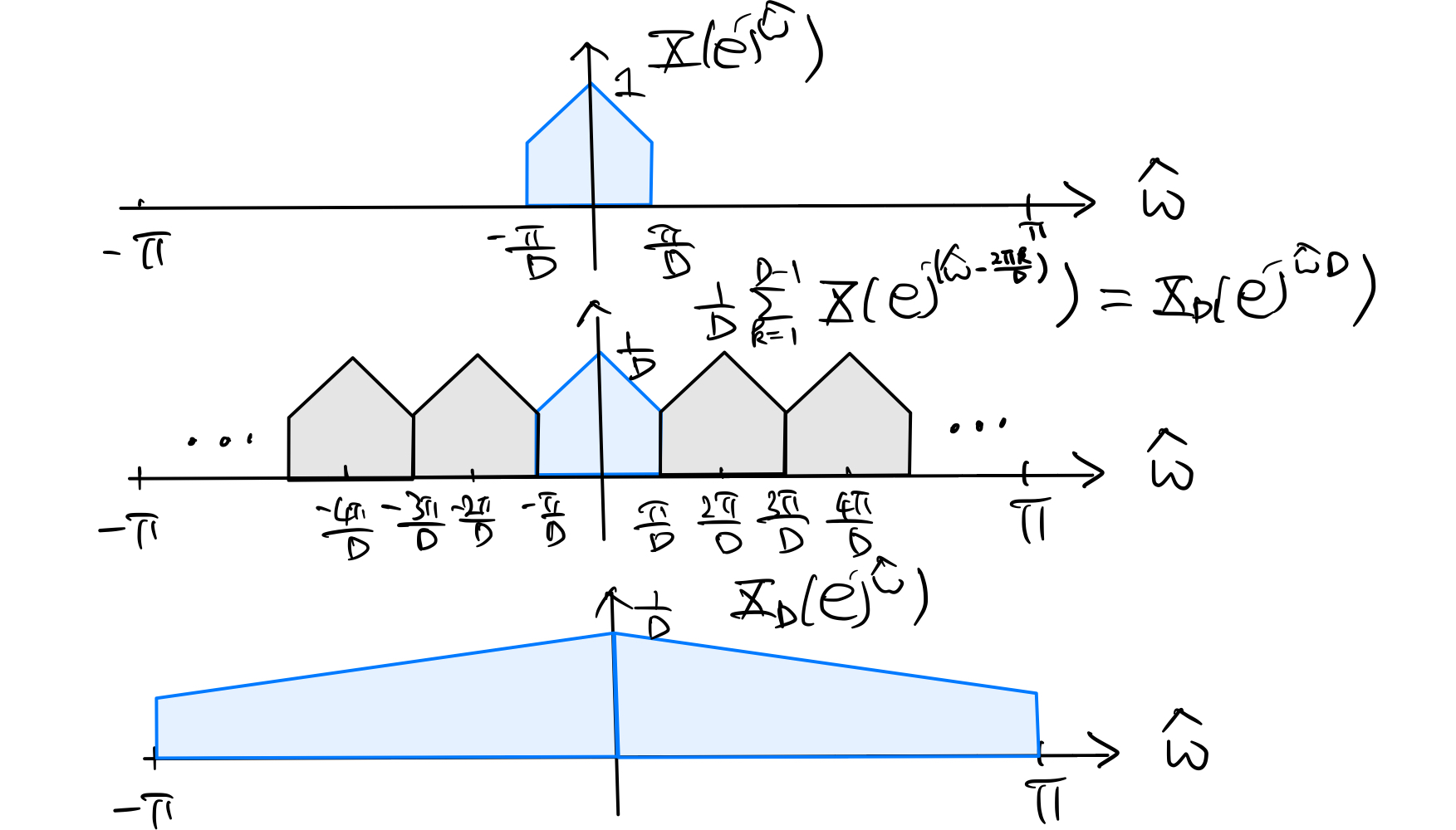
From the figure, it is clear that \(X_D(e^{j\hat\omega}) = \frac{1}{D} X(e^{j\frac{\hat\omega}{D}})\). Hence, we can get \(x[n]\) back from the downsampled signal \(x_D[n]\) by reversing the sequence of frequency-domain operations as shown in the figure above. That is, \(\displaystyle X(e^{j\hat\omega}) = \begin{cases} D X_D(e^{j\hat\omega D}) & \text{for } |\hat\omega| < \frac{\pi}{D} \\ 0 & \text{for } \frac{\pi}{D} \leq |\hat\omega| \leq \pi. \end{cases}\)
Performing the recovery of \(x[n]\) from \(x_D[n]\) in the time domain is the process of interpolation, which will be discussed in Section 7.2 next.
Undersampling \(X(e^{j\hat\omega}) \neq 0\) for \(\frac{\pi}{D} \leq |\hat\omega| \leq \pi\):
The folded spectrum \(X_D(e^{j\hat\omega D})\) for this case is illustrated in the figure below:
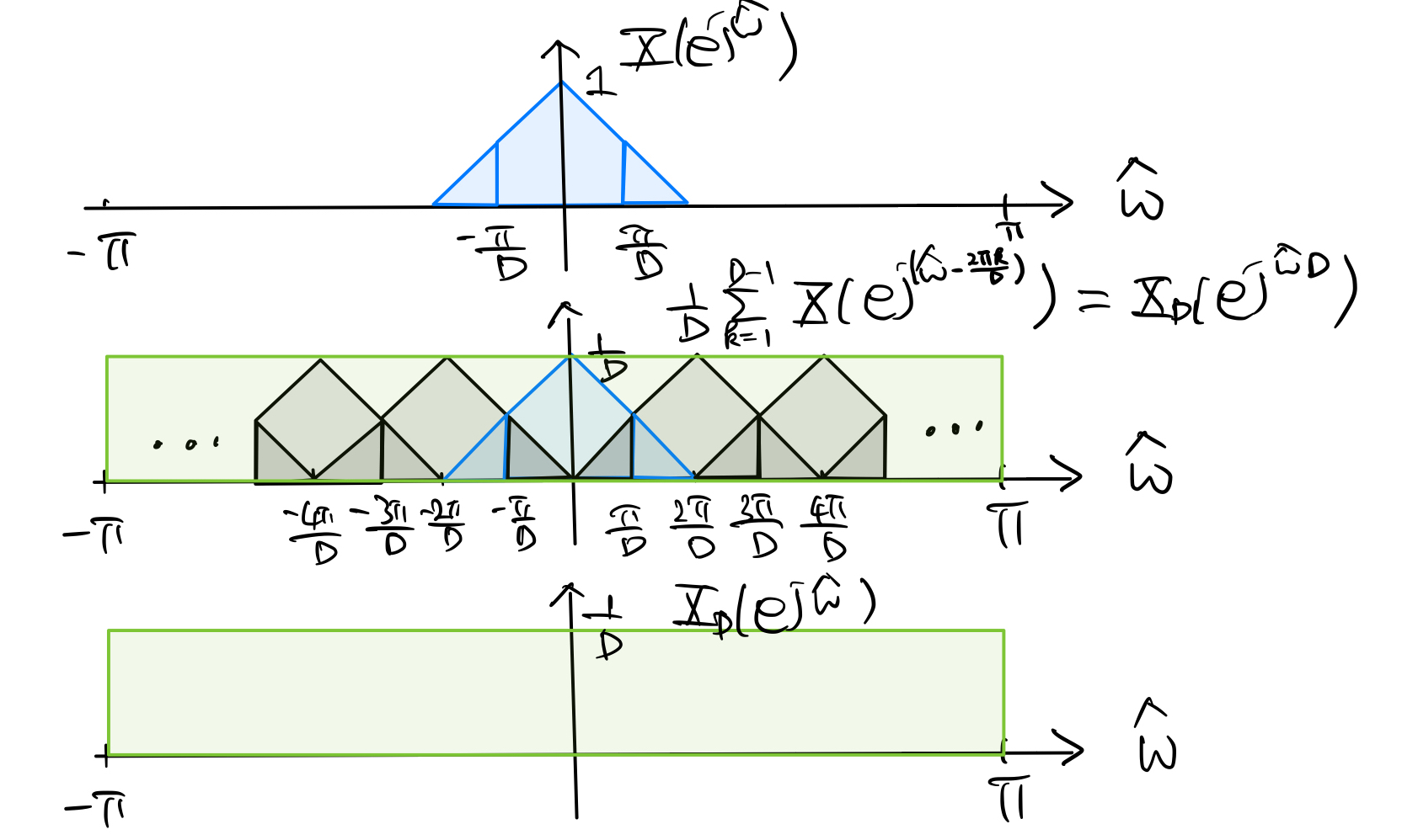
From the figure, we see that \(X_D(e^{j\hat\omega}) \neq \frac{1}{D} X(e^{j\frac{\hat\omega}{D}})\). That is, we suffer from aliasing. We may want to apply the idea anti-aliasing filter with frequency response \(\displaystyle H_D(e^{j\hat\omega}) = \begin{cases} 1 & \text{for } |\hat\omega| < \frac{\pi}{D} \\ 0 & \text{for } \frac{\pi}{D} \leq |\hat\omega| \leq \pi \end{cases}\) before downsampling in this case to control the detrimental effects of aliasing.