Overlap Save Algorithm

3.2. Overlap Save Algorithm#

In order to implement filtering operations in the frequency domain using FFT, the FFT size must be at least as large as the output length so that circular convolution implemented by FFT becomes linear convolution. This requirement is often not practical since the input length is usually very large leading to an excessive FFT size. A common solution is to divide the input signal into blocks and perform frequency-domain filtering on each block in sequence.
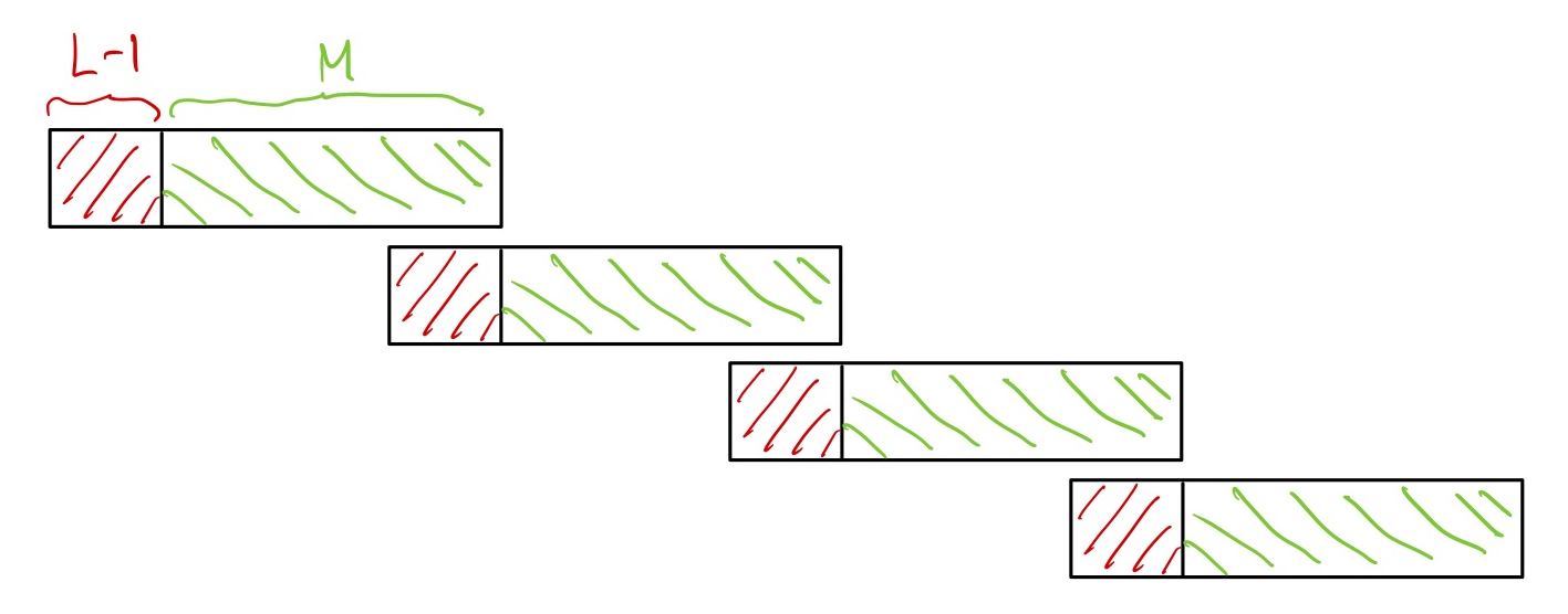
There are two main approaches, namely the overlap-add and overlap-save algorithms, to do block-wise frequency-domain filtering. Here, we focus on the overlap-save algorithm because it fits the batch FFTW3 implementation of FFT in fft.hpp better.
Let \(L\) be the length of the filter’s impulse response. Pick an FFT size \(2^m \geq L\). Then performing frequency-domain filtering on a block of \(2^m\) samples does circular convolution between the input block of samples and impulse response of the filter. The first \(L-1\) samples of the output block are corrupted due to circular convolution while the last \(M = 2^m-L+1\) samples in the output block are “clean” in the sense that they are the same as those given out by linear convolution. Hence, by overlapping consecutive blocks of \(2^m\) samples by \(L-1\) samples and then concatenating the last \(M\) samples of each successive output block, we will be able to implement linear convolution between the long input sequence of samples and the filter’s impulse response. This simple idea employed in the overlap-save algorithm is summarizes in the figure below:
It remains to choose the FFT size \(2^m\). Since we must discard \(L-1\) output samples every FFT block, we would want \(2^m \gg L\) to minimize the overhead incurred in discarding the output samples. On the other hand, the computational complexity (e.g., by counting the number of multiplications performed) of doing direct linear convolution and the overlap-save algorithm on a block of \(M\) input samples are \(\mathcal{O}\left( L M\right)\) and \(\mathcal{O}\left( m \,2^m\right)\), respectively. Hence, we would also want \(m \ll L\) in order to gain the computational advantage offered by FFT. Putting these two considerations together, a good rule of thumb to choose the FFT size is:

\[\begin{equation*} m \ll L \ll 2^m. \end{equation*}\]

Clearly, no FFT size can satisfy the condition above if \(L\) is small (say \(L < 32\)). In such case, it may simply be more computationally efficient to implement a direct linear convolution.
The class FilterOverlapSave in filters.cpp gives an example implementation of the overlap-save algorithm using the fft wrapper in fft.hpp. This implementation supports both single-rate and multi-rate filtering (see next section). To use the single-rate implementation:
1. Instantiate a FilterOverlapSave object using the single-rate constructor:
```
// Construct single-rate OverlapSave filter object
FilterOverlapSave filter_osa(in_len, L, h, nthreads);
```
  where in_len=length of input sample sequence, h=pointer to impulse response array, and nthreads=number of threads to use in FFT calculations.
2. Set the first \(L-1\) samples to the filter input to \(0\):
```
filter_osa.set_head(true);  // reset=true
```
  if filtering the first sequence of samples in a continuous flow of samples. Otherwise, copy the tail \(L-1\) samples from the previous filter input to the head \(L-1\) of current filter input to set up the correct boundary condition for continuous filtering:
```
filter_osa.set_head(); // reset=false by default
```
3. Do filtering:
```
filter_osa.filter(in, out); 
```
  where in=pointer to filter input array of length in_len, and out=pointer to filter output array. The length of out can be obtained by calling filter_osa.out_len().
For a usage example of the FilterOverlapSave class see test_filters.cpp.